How To Implement Dense_Rank() In Excel Sheet

RANK(), ROW_NUMBER() and DENSE_RANK() are three useful functions in SQL query for ranking purpose.

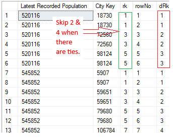
RANK () returns the rank of each row within the partition of a result set. The rank of a row is one plus the number of ranks that come before the row in question. RANK provides the same numeric value for ties For example: 1,2,2,4, 5. The numbers in ranking are not consecutive, there is gap if there are ties.

ROW_NUMBER and RANK are similar. ROW_NUMBER numbers all rows sequentially (for example 1, 2, 3, 4, 5). DENSE_RANK() returns the rank of each row within a result set partition, with no gaps in the ranking values. The rank of a specific row is one plus the number of distinct rank values that come before that specific row.

By running the T-SQL script in SQL server as below, I got the results that 2 and 4 were skipped due to the ties with RANK(); ROW_NUMBER() gave the consecutive numbers for each row within the result set partition. DENSE_RANK() gave out the rank without gap.

SELECT 
        [Latest Recorded Population]
        ,[City Key]
        ,RANK() OVER( PARTITION BY [Latest Recorded Population] ORDER BY [City Key]) AS rk
        ,ROW_NUMBER() OVER(PARTITION BY [Latest Recorded Population]  ORDER BY [City Key]) AS rowNo
        ,DENSE_RANK() OVER (PARTITION BY [Latest Recorded Population]  ORDER BY [City Key]) AS dRk
FROM [Kineteco].[dbo].[Cities]

However in the excel, DENSE_RANK is not supported directly. But it could be solved through the formula. Let me use the data set from the post Piano Exam Preparation Analysis Report.

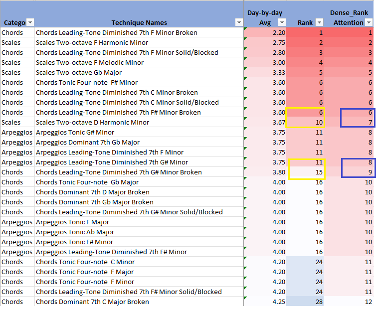
In the formula, there are 2 functions Frequency and Sum to implement ranking without skipping the number. In the chart below, there is a gap in the yellow rectangles because of using rank() function, but there is no gap in the blue rectangles because of using the formula.

I break the formula of the cell AI11 into 6 steps.

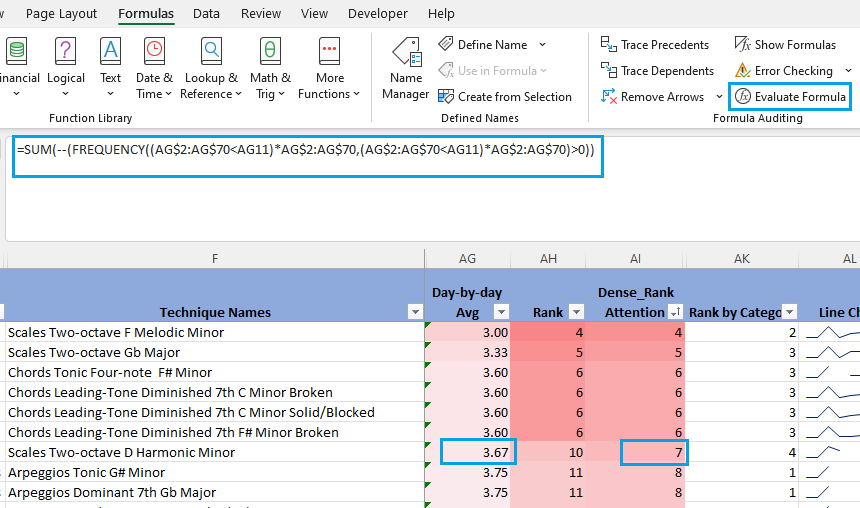
When the cursor in the cell AI11, click the formulas tab on the ribbon, then click the “Evaluate Formula” button, it will appear as:

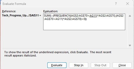
I could check the return value of each step by clicking the evaluate button.

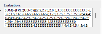
In step 1, AG$2:AG$70 is the array that includes all the average scores in column AG. AG$2:AG$70 < AG11 will find the value from the array that smaller than the value in cell AG11 which is 3.67 and will return true or false.

(AG$2:AG$70< AG11)* AG$2:AG$70 returns the values are smaller than 3.67. If the value is greater than 3.67, it returns 0. See those values from the screenshot below:

Step 2 is as same as step 1 and it returns the same result.

Step 3 is to find the frequency of the values from step 2 in the array of step 1, and return the array.I put them in the table for using understanding.

Avg Score (step2)	Frequency (step3)
2.2	1
2.75	1
2.8	1
3.1	1
3.333..	1
3.6	4
0	60
….

In step 4, it returns True or False, if the value of step 3 is greater than 0 or not.

Avg Score (step2)	Frequency (step3)	> 0 (step4)
2.2	1	True
2.75	1	True
2.8	1	True
3.1	1	True
3.333..	1	True
3.6	4	True
0	60	True
….

In step 5, use double minus to convert true and false into 1 and 0.

Avg Score (step2)	Frequency (step3)	> 0 (step4)	– (step5)
2.2	1	True	1
2.75	1	True	1
2.8	1	True	1
3.1	1	True	1
3.333..	1	True	1
3.6	4	True	1
0	60	True	1
….

In step 6, SUM() adds up all the 1 and 0 from step 5 and returns 7. So 3.67 ranks 7 among array AG$2:AG$70.

Well, this formula is just as DENSE_RANK() from SQL to implement ranking without gap for ties in excel.